This section will show you how to focus attention on a subset of your data and how to manipulate it with mathematical tools to obtain new data or improve the existing one.
In general, when you import a data set in Xplot, what you see in the drawing area is a subset of the imported data. When you apply a tool from the Xplot window (like, for example, Xplot>Calculations>Derivative), it is applied to the active data , which, in many cases, is the data you see in the drawing area, but not always. Let us define some terminology that will help us in further explaining Xplot actions:
Xplot data is all data that is already available or will be available to Xplot. Xplot data may be in a single file or in multiple files. For example, our file tmp.dat is Xplot data. If I create another similar file tmp2.dat to be used in Xplot (to overplot data to tmp2.dat), the Xplot data is everything contained in both files. A typical SPEC file usually contains many blocks of data (called scans). All data in one (or many) SPEC file are Xplot data. Xplot data is structurated in data sets, or simply sets.
A set is an array or matrix containing N points (or rows) and M columns. Our file tmp.dat contains a single set, with two columns. A SPEC file usually contains many sets (or scans). When a set is loaded in Xplot (usually by Xplot>File>Load data file you can manipulate it using the Xplot controls. It is called current set.
The current set has at least two columns, but may have more. You can display X-Y graphs of the current set by assigning a column to X and another column to Y. This is done with the display column boxes (or pulldown menus) at the bottom of the Xplot window. If you change the column number, which index starts with one, you must press <enter> to validate and tell Xplot to update. However, you can restrict the view of the X and Y data of your current set. For example, you can change the limits of the plot (using Xplot>Edit>Limits>Set Limits and Styles&ldots;) or simply by selecting part of the plot and applying the zoon button (click "Zoom Out" button to unzoom).
Sets are important to create compound plots of several curves. For that you should use the "Save Plot" button.
Plot attributes: they are characteristics of the plot that are not included in the data itself, like color, thickness, plot limits, etc.
Selected data: Click and drag the mouse over the wanted region in the drawing area. You selected an X and Y interval in the plotted data. The selected limits appear in the Xplot message. We call ”r;selected data” the points of the current set with X values in that interval.
Active data: they are the data to be used for the data analysis operations. The active data contains the points included in the X limits defined in the Xplot>Edit>Limits section. The default is that all points are active data. However, you can define manually your limits using Xplot>Edit>Limits>Set limits and Styles&ldots; In some cases, it is easier to set the limits by selecting data and then using Xplot>Edit>Limits>Set Limits as Selection Area. You can always go back to default limits by using Xplot>Edit>Limits>Set Defaults
For example, to create a plot from data in two different files tmp.dat and tmp2.dat, load first tmp.dat. The current set now is the two-column data in tmp.dat. Manipulate it if you want (change color to red, line thickness to 5, etc) and then press ”r;Save Plot” button. Apparently nothing happened. You only see at
the message line: ”r;1 Saved sets”. This means that the set you manipulated is saved to some kind of background state, becoming present, but inactive. So, what is the current set now? The answer is: an identical copy of the saved one. Now, create the next file tmp2.dat like:
; this is a comment:
; example of data to test Xplot
9 10
10 15
11 11
12 25
13 30
14 23
15 10
16 1
17 25
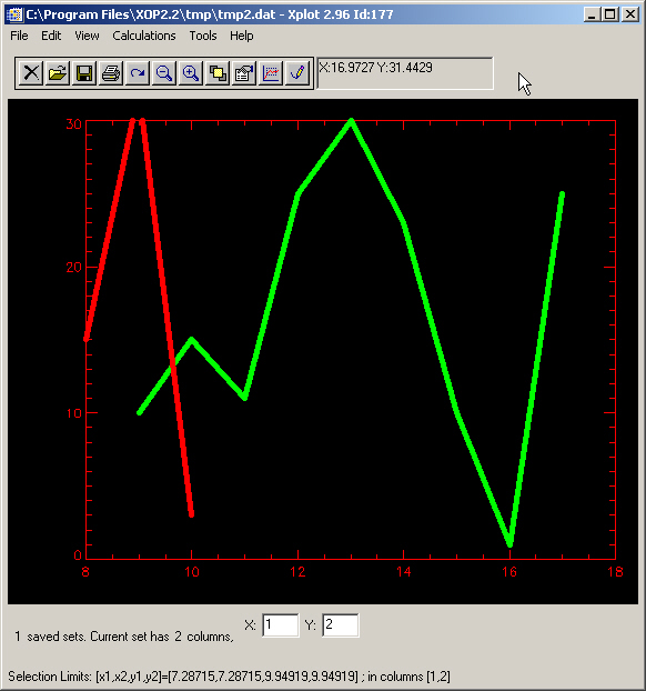
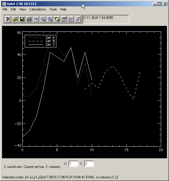
and load it in Xplot using Xplot>File>Load Data File&ldots; What happened? To see more clearly what happened, change the line color to green (index 3). You obtain:
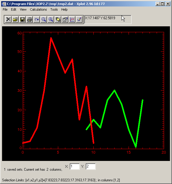
You see in green the new loaded file. You see in red the old saved set (only part of it, because Xplot automatically sets the plot limits adapted to the current set). Any operation you do in Xplot will be applied to the current set (green). May be this resulting plot is not what you wanted. You can change the limits by hand to make both sets appear in the drawing area, by using Xplot>Edit>Limits>Set Limits and Styles&ldots;I clicked the button "Clip all data" to put all data within the drawing area:
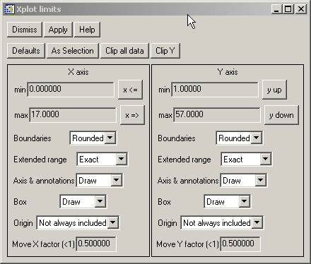
and this is what I get:
Note that Xplot rounds the limits in order to present a good looking plot. If you really want the plot in the Y interval [0,57], just set ”r;Boundaries: exact” in the Limits window.
With Xplot, you can overplot many curves by iteratively loading and
then using the ”r;Save Plot” button to keep them. Attributes
for a saved curve cannot be modified. To modify them you should pass the
saved curve to the current set, using the Plot Manager button  .
The plot manager also permits to delete saved sets.
.
The plot manager also permits to delete saved sets.
To focus the attention in some part of the plot, first select it. For that, click and drag the mouse over the wanted region. The selected limits appear in the Xplot message line. The selected area is useful for three things:
Zoom it. Press the Zoom button  to adjust the plot boundaries to the selected
area. Press
to adjust the plot boundaries to the selected
area. Press  to go back the original plot. Note that after zooming out, the
selection is not lost: click button again, and you will see again the
zoomed plot.
to go back the original plot. Note that after zooming out, the
selection is not lost: click button again, and you will see again the
zoomed plot.
You can define the limits of the plot to the selected area, by choosing Xplot>Edit>Limits>Set Limits as Selection Area. The limits are then fixed and even if you load a new data set, they will not change. To change manually the limits, use Xplot>Edit>Limits>Set Limits and Styles&ldots; To tell Xplot to adjust the limits automatically to the current set, select Xplot>Edit>Limits>Set Defaults.
Information of selected area is passed to two ”r;Edit” operations:
i) Xplot>Edit>Data&ldots; allows you to modify and remove points. When you select this option, the selected points will be highlighted.
ii) Xplot>Edit>Cut&ldots; allows you to remove undesirable parts of your current set. The default limits presented here are adjusted to the selection area. Note that the defaut limits (automatic limits adjustment) is manifested in the Xplot>Edit>Limits>Set Limits and Styles&ldots; window with the same numerical value for the min and max (usually zero).
The active data for the data analysis (most operations in the Xplot>Calculations menu) is the selected X and Y columns in the current set, in the interval selected by the plot limits (check them with Xplot>Edit>Limits>Set Limits and Styles&ldots;). This means that a typical operation (e.g., derivative) will be applied only to the X-Y data in the current set in the [xmin, xmax] interval set in Xplot>Edit>Limits>Set Limits and Styles&ldots;
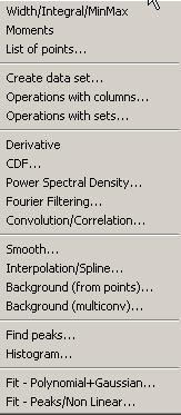
There are many operations that can be applied to the active data in Xplot. There are under the Xplot|Calculations menu:
Remember that:
The active data for the data analysis (most operations in the Xplot>Calculations menu) is the selected X and Y columns in the current set, in the interval selected by the plot limits (check them with Xplot>Edit>Limits>Set Limits and Styles&ldots;).
Statistics:
Width/Integral/MinMax: Calculates the full width at half-maximum (FWHM), extrema and integral of the active data. You can optionally write some of these values as a plot Legend. Integration is done by using the INT_TABULATED IDL routine.
Moments: Calculate the moments (mean, variance, skewness, kurtosis, mean absolute deviation and standard deviation) of the current data. It uses the MOMENT function
Data manipulation (creating and combining data):
List of points: create a list of points (X,Y) by by clicking iteratively with the mouse. The output is written to a file for further use.
Create data set&ldots;Allows to easily create a set of data by defining the abscissas interval and a formula for the ordinates.
Operations with columns&ldots; & Operations with sets&ldots;These options, because of their importance, are explained in detail in the next sections.
Derivative/Integral-based operations
Derivative: This options created a new Xplot window with the derivative of the current data. It uses the DERIV function of IDL.
CDF&ldots;
This options created a new Xplot window with the Cumulative Distribution
Function (CDF) of the current data. This function is the inverse function
of the derivative. For example, applying first the derivative and then
CDF to your data you should go back to the original data. The calculation
is done calling the INT_TABULATED function a number of times equal to
the number of abscissa points. The CDF function of a given signal f(x)
is defined as:
Powel Spectral Density&ldots;This option computes the power-spectral-density function from the active data. It is defined as: PSD=(Xmax- Xmin)*ABS(FFT(Y),-1)^2. Note that the use of FFT implies that the abscissa points must be equi-spaced.
Fourier Filtering&ldots; This option permits interactive Fourier filtering of the current data. When you call this option, a new window appears, showing three displays: one with the original signal, one with the filtered signal and another one with the filtering window used. You can select different Filter Functions, Filter Order, Filter Type and values of Frequency cutoff and Bandwidth. Open for example these option from Xplot holding the sinusoidal data from last section. Play with the Frequency Cutoff function and you will see how you can filter the high frequency component (with cutoff values below 20, approximately). You can save the displayed values to file(s) by using the File>Save as (New ASCII FIle)... option from the menu bar, and then the filtered data can be re-injected in Xplot for further manipulation.
Convolution and Correlation&ldots;This option permits to calculate convolution and correlation between two data sets, A (the current set) and B. The set B can be one of the following cases:
1) B=A autoconvolution/autocorrelation cases.
2) B from an external file.
3) B a Gaussian, Lorentzian or a liner combination of both (the so-called pseudo-Voigt function: v(x)=r*L(x)+(1-r)G(x), with r the ratio or linear coefficient between Lorentzian and Gaussian).
The Convolution and correlation are calculated from:
CONV(x) = integral( A(y) B(x-y) dy);
CORR(x) = integral( A(y) B(y-x) dy).
Of course, CONV(x) = CORR(x) if B(y) is symmetrical. The program interpolate both curves (using INTERPOL) to the biggest interval and smallest step between both abscissas and convolute/correlate them).The result may be normalized. The program uses the FFT method to perform the calculations
Interpolation/Smooth/Background substraction
Smooth&ldots; The Xplot smooth option smooths the Y data of the active graph. Two methods are available:
i) Boxcar average: the results are a current set smoothed with a boxcar average of the specified width. Xplot uses the SMOOTH function of IDL for the Boxcar method.
ii) Least Squares: the results are a current set smoothed applying a least squares smoothing polynomial filter also called Savitzky-Golay smoothing filter. Xplot uses the POLY_SMOOTH routine of Frank Varosi for the Savitzky-Golay method.
Interpolation/Spline&ldots; This options creates a new Xplot window with interpolated data. This option is normally used to create a new set of data with the same look than the original, but with a different number of points. Three possible interpolations are possible: i) Linear Interpolation (using INTERPOL from IDL). ii) Spline interpolation (using SPLINE from IDL). This option asks for the TENSION value. The default value is 1.0. If TENSION is close to 0, (e.g., .01), then effectively there is a cubic spline fit. If TENSION is large, (e.g.,greater than 10), then the fit will be like a polynomial interpolation. iii) Parametric Spline (using SPLINE_P from IDL). Here the number of points of the result is defined by the program itself.
Background (from points): This option substracts a background it from current data. First, you have to create a file with the background ("List of points"can be used for that).
Background (multiconv): Computes the background by an iterative procedure. In each iteration, the signal is convoluted with a kernel. For each point the signal is replaced by the convolution value, only in the case that the latter is larger. It uses the function mConvBackground()
Miscellaneous
Find peaks. Two methods are proposed:
1) Based on first derivative: i) calculate first derivarive ii) smooth it (with parameters m,z) iii) search for points with zero derivative (peak candidates)iv) calculate the maximum amplitude (delta_max) of the derivative data when going through a zero value, v) comparison of each amplitude (delta) of the derivative data when trought a zero value with delta_max: if (delta/delta_max > theshold) :=> Peak
2) Based on second derivative: i) calculate second derivarive S of y ii) smooth it (with parameters m,z) iii) Take the negative part of S and calculate the absolute value |S| iv) Calculate the intervals where |S| is clipped by zeroes. v) Take a peak candidate in each interval (the point with highest y value) vi) if |S|>t*F :=> Peak, with: F is the standard deviation of F, t is a normalised threshold, i.e., it gives the maximum number of peaks for t=0 and no peaks for t=1.
The Number of Peaks is not linear with the threshold. For selecting adequated theshold values the possibility of analysing the threshold (plot of Number of peaks versus threshold value) is also available. References: M.A. Mariscotti, Nucl. Instrum. Meth. 50 (1967) 309-320; Documentation of FullProf code, Juan Rodriguez-Carvajal. For more information see the doc in routine PeakFinder.
Histogram&ldots; Makes histograms from one column of the displayed data. Note: for displaying data in histogram style, use "Shw Controls"windows, and select Symbol: 10 Histogram.
Fits:
Polynomial+Gaussian: makes a fit of the current set with a function made by a polynomial, gaussian or a combination of them.
Peaks. Non-linear. Exports data to the FuFiFa application, for non-linear fit.
This option allows you to calculate a new column data in the current set as a function of the existing ones. The result can:
be appended to the set, thus substituting the current set by a new one with one more column.
substitute an existing column in the current set.
be exported to a new Xplot window.
The user has to type in the pop-up window the expression in IDL syntax to create the new column data. This expression has variables names named as col1, col2, etc. for referring to the existing columns in the current set. After the column operation the old X and Y columns are still displayed. You have to change manually the Y column to visualize newly created data (in the case that data is not overwritten to the same column).
This option allows you to do a lot of data analysis and data reduction operation on your data. For example, you can try with the data of tmp.dat some column expressions (supposing currently display X is col1 and Y is col2) (consider the new created column as a new Y column, unless specified otherwise):
Normalization of the peak value to 10: col2/max(col2)*10
Normalization of Y column data between in the Y interval [0,1]: (col2-min(col2))/(max(col2)-min(col2)
Substract a straighth line Y=2X+3: col2 &endash; (2*col1+3)
Shift data vertically 10 units (vertical translation): col2+10
Shift data horizontally 5 units: col1+5 (the new created column is now X)
Average columns 2 to 4: (col2+col3+col4)/3
Square of column X: col1^2
Natural logarithmic of column 1: alog(col1)
You can also type your expression as a function of other IDL functions.
This option allows you to create a new two-column set of data (which will be named C), as a function of the X and Y columns of the current set (that we call set A), and an optional two-column set (called B) that is sitting in a disk file. The user must provide an expression to create the abscissas and ordinates of the new set C (named Cx and Cy, respectively). This expression has to be written in IDL syntax, and is a function of the abscissas and ordinates of the data sets A and B (with abscissas Ax and Bx and ordinates Ax and Ay).
In the case that the abscissas of the A set (Ax) is different from the newly created Cx, then the A data set is interpolated to fit in the new grid Cx. The same happens for B, if two sets are selected.
An example: load the file tmp.dat in Xplot, call Operations with sets... option and type in the input data window the following parameters: Cx = Ax*1.0, Cy = Ay+By, Number of data sets: 2, A data set: current set, B data file: tmp2.dat (you may also type "?"and a file browser will allow you to select the corresponding file, Write output to file: No, Overplot original data: Yes. These inputs mean that we want to create a new set C with abscissas values the same as the original one (Cx=Ax), and the ordinates value is Ax plus 2 times Bx, there B is a set defined in the tmp.dat file (in this example the sets A and B are the same, but is evident that B may be a file with any data). The input data window and the resulting new window with the resulting data (after clicking the Accept button) looks like:
In the new window you can see three data lines: The resulting one plus the original ones (as requested). Some values of set C are a bit different from the originals (set A) due to the contribution of the extrapolated set B. If you would like that the abscissas of the result will cover the full range, use Cx=[Ax,Bx], or Cx=MergeArrays(Ax,Bx).
The ”r;Operations with data set” option can also be used to create data from scratch in Xplot. For that you may use the IDL function FINDGEN(N), that creates an array of N points starting from 0 and ending in N-1. Or, use the MAKEARRAY1 function, for example: Cx=MakeArray1(100,2.0,90) which will define Cx as an float array of 100 points from 2 to 90. You may operate with that in order to define the abscissas values (Cx), and then define the ordinates (Cy) as a function of Cx. Instead of that, you could also use the option: Xplot>Calculations>Create data set&ldots;
You can do sophisticated analysis by creating an XOP macro. This is a sort of program that is interpreted line by line. You can use it to create and manipulate your data, to make iterative data analysis, etc. You can call XOP macro from Xplot>Tools>XOP Macro and optionally you can input the current plot in Xplot.
You can also call Xplot from an XOP Macro.