Xplot2D contains several tools for the analysis of diffraction (or small angle scattering) images. It can be x-ray, neutron or electron diffraction. In order to extract useful information from the image, we must know some parameters related to the geometry of the detector and sample position. Xplot2D permits to obtain (and refine) these parameters starting from a reference compound.
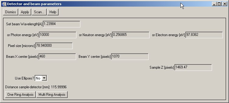
Select "Diffraction>Select detector and beam pars...". You will get a window in which you could define some of the parameters of your measurement. For example, we know that our image is an x-ray diffraction image measured with a camera with a pixel dimension of 78.94 mm, the photon beam had an energy of 10000 eV and the distance detector-sample is about 11.6 cm. We fill these values, select "Use ellipses=No" (this means that we suppose that the beam is orthogonal to the detector, we may later correct for small non-orthogonality, but it is a good idea to start like that). Nothe that the detector distance must be entered in pixels so we put 116/0.07894=1467.97. Also, we placed rough values of the beam center (center of the rings) that we may obtain pointing to the center and copying the cursor values. We get:
Now we want to overplot rings that correspond to the position of the peaks in the diffractogram of our reference (quartz). For that you should prepare a multicolumn file with at least two columns. In the first column place either the d-spacing or 2q values of the peak positions. In the second column place the peak intensity (arbitrary units). In the third column you may place a color index, starting by 2. This allows you to overplot different phases each one with a different color.
For example, the d-spacing of reference powder compounds can be obtained from a multitude of sources. They can be classified in two:
Databases containing a list of d-spacing for the references. The most well known is the PDF (Powder Diffraction File) database (commercial).
Cell refinement data. Some databases contain the structure of the compounds from which it is possible to calculate the list of d-spacing. Some examples
The XOP application XPOWDER may help to prepare this information
For this example, I used the program POWDERCELL to compute the d-spacing list using its example "quartz". The result is in the quartz.dspacing file that you can find in the "examples" directory of the XOP directory structure.
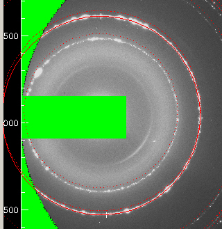
Load this file using "Diffraction>Overplot rings...". You will see some red rings overplotted on your image. You may recognise that they correspond to your image structures, but they are not well aligned with the image rings.
A first alignment ”by eye” should be done by changing manually the parameters in Diffraction->Define detector and beam pars&ldots; window and play with the parameters of the image center and distance D in order to get a good matching of the overplotted rings with your image’s rings. However, you can use the automatic tools that follow.
Let us try to optimize the detector and beam parameters for having a "perfect" match of the overplotted rings with our image of the reference compound.
A first step should be to optimize parameters using only one ring. Use "ROI/Mask>Circle>3 points on the circle with mouse" to select a circular ROI that should match, let us say, our image second inned circle:
Then, in the detector and beam parameters window ("Diffraction>Select
detector and beam pars...") click  . You will see an annulus contouring your
circular ROI, and a question related to use the annulus of the selected
ROI for the calibration. Select "No" for using the circular
ROI. Another window proposes you the d-pacing corresponding to this ring.
Xplot2D takes it from the quartz.dspacing file, and selects the closer
d-spacing to our selection. However, you must check it is correct, and
eventually change it. Another dialog window will ask you about the optimization
starting parameters. Answer "No" to start with the current parameters
defined in the window "Diffraction>Select detector and beam pars...".
Accept the new parameters and you will get:
. You will see an annulus contouring your
circular ROI, and a question related to use the annulus of the selected
ROI for the calibration. Select "No" for using the circular
ROI. Another window proposes you the d-pacing corresponding to this ring.
Xplot2D takes it from the quartz.dspacing file, and selects the closer
d-spacing to our selection. However, you must check it is correct, and
eventually change it. Another dialog window will ask you about the optimization
starting parameters. Answer "No" to start with the current parameters
defined in the window "Diffraction>Select detector and beam pars...".
Accept the new parameters and you will get:

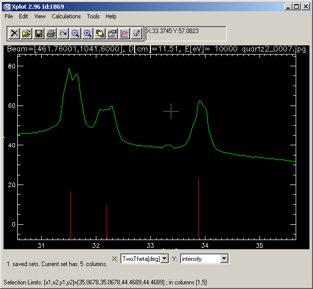
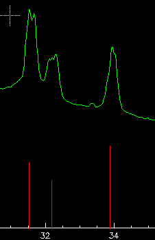
It looks nice: the overplotted rings fit well with the image structures. However, it is not good. For a proof, calculate the corresponding diffractogram, using "Diffraction>Azimuthal integration (isolated window)" and make a zoom on some peaks, you will see that although the peaks are well positioned, the shape is not "nice", because i) The paremeters can be further refined, and ii) one should also consider corrections for non-orthogonality. You get something like:
Next step is to use  . Try it and accept all dialogs. In a first
step, you will see an annular region around each ring. The program extracts
the pixels within these annuli (the width of the annuli can be changed
using the ROI/Mask Manager, annulus tab), make some binning (calculates
the center of mass for a number of azimuthal sectors, which number is
defined in "Edit>Preferences...", and applied a non-linear
optimization algorithm to optimize the detector+beam parameters to the
experimental data. The diffractogram calculated after accepting these
new parameters still present some strange features in the peaks, which
are probably due to non-orthogonality effects:
. Try it and accept all dialogs. In a first
step, you will see an annular region around each ring. The program extracts
the pixels within these annuli (the width of the annuli can be changed
using the ROI/Mask Manager, annulus tab), make some binning (calculates
the center of mass for a number of azimuthal sectors, which number is
defined in "Edit>Preferences...", and applied a non-linear
optimization algorithm to optimize the detector+beam parameters to the
experimental data. The diffractogram calculated after accepting these
new parameters still present some strange features in the peaks, which
are probably due to non-orthogonality effects:
Select now "use ellipses=Yes" and repeat the multi-ring analysis to try to improve the calibration. You may easily forget some rings during the optimization placing a -1 in the "flag"of the displayed list. This is a good idea for the outer rings, because data here is quite scarce. With some iterations in this way, playing with the "flag" and eventually changing the annuli width, one should obtain satisfactory results. In our case, data is not very good because the sample is not a very fine powder and produces strong spots in the image. Additionally, we ate using a jpg file therefore loosing much statistics.
You can also perform a scan of a given parameter. For that, click  in "Diffraction->Define detector
and beam pars&ldots;".
in "Diffraction->Define detector
and beam pars&ldots;".
We already performed this important operation to produce a diffractogram from a diffraction image. The azimuthal integration can be displayed in a "new isolated window", which means a window that stays idle until you kill it, and in an autorefresh window. The latter is a window that displays the recalculated diffractogram each time that Xplot2D is refreshed, that means each time you load a new image, change some beam or detector parameter, etc.
Now, you simply read a new image, and the windows will be updated with
the data (and integral) from this image. However, you should apply the
current mask to the new loaded image. For that, set (Fig
2). Window File-> Set load image properties&ldots; YES to Apply current
mask. If you want to visualize a number of consecutive images, it is very
useful to use the  (
( ) button that will increment (decrement) the file
index.
) button that will increment (decrement) the file
index.
If you want to integrate a collection of images, just select YES in save azimuthal integration [file xplot2d.azi]. Once you set that, every integrated profile will be added to the xplot2d.azi file, in your current directory. This is a file of SPEC type, and each profile is added as a new scan.
Then in Xplot2d File->Load Image&ldots; and make a multiple file selection (using the <shift> and/or <ctl> Keys). Note that this multiple selection is only working with EDF or MAR files. Xplot2d will load sequentially the files, calculate the integral, and write it to the xplot2d.azi file. The user is responsible of renaming this file and storing it in a safe place. This xplot2d.azi file can be visualized and further processed using Xplot or EXODUS.